Training deep neural networks on CPUs is difficult. This tutorial will guide you on how to fine-tune VGG-16 net using Keras on Google Colaboratory, which is a free GPU cloud platform. If you are new to Google Colab, this is the right place for you and you will learn:
- How to create your first Jupyter Notebook on Colab and use a free GPU.
- How to upload and use your custom datasets on Colab.
- How to fine-tune the Keras pre-trained model (VGG-16) in the Foreground Segmentation domain.
Now, let’s get started…
1. Create your first Jupyter Notebook
Suppose that you have already logged in to your Google account. Please follow these steps:
a). Navigate to http://drive.google.com.
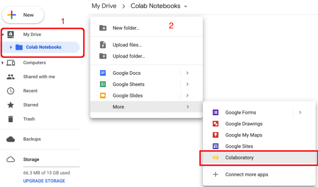
b). You will see My Drive tab on the left pane. Now, create a folder inside it, say Colab Notebooks.
c). Right-click somewhere else on the right pane inside the created folder, select More > Colaboratory. Another window will pop-up and you can name your notebook to something else, say myNotebook.ipynb. Cheer!!! You have created your first notebook on Colab.
2. Set a GPU accelerator for the notebook
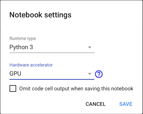
In the notebook, select Runtime > Change runtime type. One window will pop up. Then, choose your runtime type, select GPU from Hardware accelerator dropdown menu and save your settings (Figure below).
3. Upload your custom datasets to Colab
You have finished setting up your notebook to run on a GPU. Now, let’s upload your datasets to Colab. In this tutorial, we work on Foreground Segmentation, where foreground objects are extracted from the background (Figure below).

There are several options in uploading datasets to Colab, however, we consider two options in this tutorial; first, we upload to GitHub and clone from it to Colab, second, we upload to Google Drive and use it directly in our notebook. You may choose either option a). or b). below:
a). Clone from GitHub
Let’s clone above dataset to the created notebook. In your notebook’s cell, run
!git clone https://github.com/lim-eren/CDnet2014
You will see something like this:

Done! Let’s list down using ! ls */train/* the training set to see if it works:
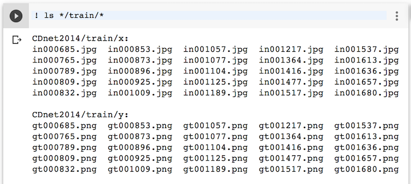
Here we go ! The training set contains 25 input frames and 25 ground-truth frames. Skip section b). and jump to section 4. if you have done this step.
b). Download from Google Drive
Another option is to upload your dataset to Google Drive and clone from it. Suppose that you have already zipped the training set above, say CDnet2014.zip, and uploaded to Google Drive in the same directory as myNotebook.ipynb. Now, right click on CDnet2014net.zip > Get shareable link. Copy file’s id and store it somewhere (we will use it later).

Then, authenticate Colab to access Google Drive by running the following codes. Follow the link to get a verification code and paste it in below textbox, then press Enter.

Then, let’s download CDnet2014net.zip file content into our Jupyter Notebook (replace YOUR_FILE_ID with the id obtained in above step) and unzip it by running the following codes:

Done! You have downloaded your dataset from Google Drive to Colab. Let’s proceed to section 4 to build a simple neural network using this dataset.
4. Fine-tune your neural network
After your dataset is downloaded to Colab, now let’s fine-tune Keras pre-trained model in Foreground Segmentation domain. Please follow the following steps:
a). First of all, add this code snippet on top of your notebook to obtain reproducible results across machines (please run the code snippets in your notebook’s cells):
# Run it to obtain reproducible results across machines (from keras.io)
from __future__ import print_function
import numpy as np
import tensorflow as tf
import random as rn
import os
os.environ['PYTHONHASHSEED'] = '0'
np.random.seed(42)
rn.seed(12345)
session_conf = tf.compat.v1.ConfigProto(intra_op_parallelism_threads=1, inter_op_parallelism_threads=1)

from keras import backend as K
tf.random.set_seed(1234)
sess = tf.compat.v1.Session(graph=tf.compat.v1.get_default_graph(), config=session_conf)
tf.compat.v1.keras.backend.set_session(sess);
b). Create a function to load data from Colab. This function returns input images (X) with corresponding ground-truths (Y):
# load data func
import glob
from keras.preprocessing import image as kImage

def getData(dataset_dir):
    X_list= sorted(glob.glob(os.path.join(dataset_dir, 'x','*.jpg')))
    Y_list = sorted(glob.glob(os.path.join(dataset_dir, 'y' ,'*.png')))

    X= []
    Y= []
    for i in range(len(X_list)):
        # Load input image
        x = kImage.load_img(X_list[i])
        x = kImage.img_to_array(x)
        X.append(x)

        # Load ground-truth label and encode it to label 0 and 1
        x = kImage.load_img(Y_list[i], grayscale = True)
        x = kImage.img_to_array(x)
        x /= 255.0
        x = np.floor(x)
        Y.append(x)
    X = np.asarray(X)
    Y = np.asarray(Y)

    # Shuffle the training data
    idx = list(range(X.shape[0]))
    np.random.shuffle(idx)
    X = X[idx]
    Y = Y[idx]
    return X, Y
c). Initial a vanilla encoder-decoder model. We adapt the VGG-16 pre-trained model as an encoder, where all fully-connected layers are removed, only the last convolutional layer (block5_conv3) is fine-tuned and the rest of the layers are frozen. We use transposed convolutional layers to recover features resolution in the decoder part.
Since it is a binary classification problem, binary_crossentropy is used and the output from the network will be the probability values between 0 and 1. These probability values need to be thresholded in order to obtain binary label 0 or 1, where label 0 represents the background and label 1 represents the foreground.
import keras
from keras.models import Model
from keras.layers.convolutional import Deconv2D
from keras.layers import Input

def initModel():
    ### Encoder
    net_input = Input(shape=(240,320,3))
    vgg16 = keras.applications.vgg16.VGG16(include_top=False, weights='imagenet', input_tensor=net_input)
    for layer in vgg16.layers[:17]:
      layer.trainable = False

    x = vgg16.layers[-2].output # 2nd layer from the last, block5_conv3

    ### Decoder
    x = Deconv2D(256, (3,3), strides=(2,2), activation='relu', padding='same')(x)
    x = Deconv2D(128, (3,3), strides=(2,2), activation='relu', padding='same')(x)
    x = Deconv2D(64, (3,3), strides=(2,2), activation='relu', padding='same')(x)
    x = Deconv2D(32, (3,3), strides=(2,2), activation='relu', padding='same')(x)
    x = Deconv2D(1, (1,1), activation='sigmoid', padding='same')(x)

    model = Model(inputs=vgg16.input, outputs=x)
    model.compile(loss=keras.losses.binary_crossentropy, optimizer=keras.optimizers.RMSprop(lr=5e-4), metrics=['accuracy'])
    return model
d). We set a learning rate of 5e-4, batch_size of 1, validation_split of 0.2, max-epochs of 100, reduce the learning rate by a factor of 10 when validation loss stops improving in 5 epochs, and stop the training early when validation loss stops improving in 10 epochs. Now, let’s train the model.
# load data
dataset_path = os.path.join('CDnet2014', 'train')
X, Y = getData(dataset_path)

# init the model
model = initModel()

early = keras.callbacks.EarlyStopping(monitor='val_loss', min_delta=1e-4, patience=10)
reduce = keras.callbacks.ReduceLROnPlateau(monitor='val_loss', factor=0.1, patience=5)

model.fit(X, Y, batch_size=1, epochs=100, verbose=2, validation_split=0.2, callbacks=[reduce, early], shuffle=True)
model.save('my_model.h5')
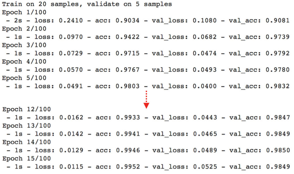
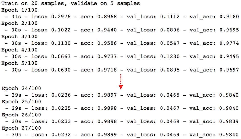
It takes around 1 second for one epoch, so fast!!! The maximum accuracy is above 98% on validation set. Not bad, right? Now, let’s pause a bit. Let’s compare the speed between training with and without GPU (you can skip this comparison and jump to the testing part if you want). To train without GPU, set the Hardware accelerator to None (refer to Section 2. above). Here are the training logs. Without GPU, it takes around 30 seconds for one epoch, while it takes only 1 second when training with GPU (about 30x faster)
Now, let’s test the trained model on test set with Colab GPU (you can run !ls */test/* to see testing frames with corresponding ground-truths).
# load test data
dataset_path = os.path.join('CDnet2014', 'test')
X, Y = getData(dataset_path)
# predict
pred = model.predict(X, verbose=1, batch_size=1)
print(tf.compat.v1.Session().run(K.mean(K.equal(Y, K.round(pred)))))
# output: test on GPU
# 10/10 [==============================] - 1s 68ms/step
# 0.98944664
Cheer!!! We can achieve 98.94% testing accuracy by just using 25 training+validation examples with a vanilla network. Note that due to the randomness of training examples, you may get similar results as mine (not exactly the same but only a small precision difference).
Note one issue: Our model is overfitting the training data, this is your job to combat this problem. Hint: Use regularization techniques likes Dropout, L2, BatchNormalization .
e). Let’s plot the segmentation mask by running the following codes:
import matplotlib.pyplot as plt
plt.rcParams['figure.figsize'] = (12.0, 9.0)

idx = 1 # image index that you want to display

img = np.empty(3, dtype=object)
img[0] = X[idx]
img[1] = Y[idx].reshape(Y[idx].shape[0],Y[idx].shape[1])
img[2] = pred[idx].reshape(pred[idx].shape[0],pred[idx].shape[1])
title = ['input', 'ground-truth', 'result']
for i in range(3):
  plt.subplot(1, 3, i+1)
  if i==0:
    plt.imshow(img[i].astype('uint8'))
  else:
    plt.imshow(img[i], cmap='gray')

  plt.axis('off')
  plt.title(title[i])
plt.show()
Here we go! The segmentation result is not bad at all! Most of the object boundaries are misclassified and this problem primarily due to the case where void labels (ambiguous pixels around the object boundaries) are considered in the loss computation during training. We can improve the performance more by omitting these void labels in the loss. You may refer to here or here on how to do so.

Summary
In this tutorial, you have learned how to use Google Colab GPU and trained the network in a fast way. You have also learned how to fine-tune Keras pre-trained model in the Foreground Segmentation domain, and you may find it interesting in your future research.
If you like this post, feel free to share or clap. Please have a nice day!

